|
| EBSD and BKD |
|
|
|
Pattern Solving
1. Indexing a Kikuchi Pattern A Kikuchi pattern can be interpreted as a gnomonic projection of the crystal lattice under the beam spot on the flat registration screen. The angles between the centerlines of bands correspond to interplanar angles of the crystal lattice, and the bandwidths correspond to the reciprocal interplanar spacings. This means that the geometry of a Kikuchi pattern is specific to the structure and the orientation of the crystallite. The bands can therefore be indexed with the Miller indices of the associated lattice planes. To do this, the bandwidths are converted into lattice plane spacings using Bragg's equation. Furthermore, the angles between the band centers are determined and these values are compared with the lattice plane spacings and the angles between the lattice planes of the crystal structure of the material to be examined. To index a Kikuchi pattern, you only need to know the positions and widths of a few bands. So the most important step in pattern solving is to precisely determine the positions of Kikuchi bands. While a skilled user can easily detect even diffuse bands on a strong background, automatic band localization is a task not so easily accomplished with software. In practice, it has proven successful to localize the bands by applying a Radon transformation to the Kikuchi pattern.
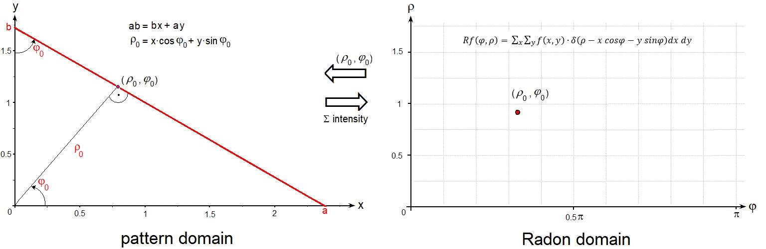
2. Radon versus Hough Transformation 2a. The Radon Transformation The statement in Johann Karl Radon's publication from 1917 is that for every direct transformation from a manifold in m-dimensional space to a manifold in n-dimensional space, there also clearly exists an inverse transformation. It was not until recently, with the development of image reconstruction in computer tomography, that the Radon transform found major practical applications. The inverse Radon transform is also particularly advantageous for the evaluation of Kikuchi patterns as it allows the simple implementation of filter functions. In the 2-dim space R2 the Radon transformation [1] is often defined as a continuous function that projects the intensity distribution f(x, y) along a line S in an image f(φ,ρ) into the 2-dim Radon space. The transformation process is defined by the line integral The digitally recorded Kikuchi pattern, however, consists of a discrete matrix f[x, y] of gray-scale image points called pixels. We must therefore consider a discrete Radon transformation, with the integrals replaced by sums. The image domain has the size of the recorded pattern, that are Mx × Ny pixels, or is binned by m × n for the sake of higher speed but at the cost of reduced accuracy. The Radon domain consist of an array of F×R
discrete cells on a Cartesian grid (φ, ρ). The size is adjusted to the angular resolution and the density of the scanned points in the EBSD measurement. The concept of Radon transformation has some advantages for band localization [2, 3]. A Kikuchi band can be thought of as a bundle of straight lines slightly rotated and shifted with respect to each other. Thus, applying the Radon transform, the intensity profile of a band is mapped pixel by pixel not to a sharp point, as would be the case with a single straight line, but smeared out in a kind of "butterfly" motif in the Radon domain. These peaks are much easier to localize than band-like motifs in the Kikuchi pattern. After the reverse transformation, the width, position and intensity profile of the Kikuchi band under consideration are known. Once at least three bands of a pattern have been determined, indexing can take place. In practice, however, considerably more bands are required to obtain a unique and reliable solution. The implementation of the inverse Radon transformation offers particular advantage in the construction of the Radon domain from the pattern. Each cell in the Radon domain is firmly correlated with a specific straight line in the pattern, whose intensity values can be interrogated directly, interpolated and rounded if necessary, accumulated and then stored in this cell. A clever approach is so to traverse the domain in Radon space inversely cell by cell (φ, ρ), instead of traversing the Kikuchi pattern and transforming pixel by pixel into a sinoidal curve in the Radon domain. Since successive points on the straight line are considered, the intensity profile along the line can be interrogated. For example, sections of the straight line have similar intensity inside a band and a cusp or a peak at the bordering Kikuchi lines. Short sections that indicate lines (partly) outside a band, can be skipped during the transformation by applying a run-length filter. Similarly, artifacts and intensity peaks ("hot spots") can be masked out by applying local bounds along the intensity profile. Locally excessive intensity values occur at the zone axes, for example, while diffraction points or dynamic diffraction effects can cause unusually high or low intensity modulations. Applying a nonlinear intensity operator to the domain [3] can further suppress noise and effectively improve contrast. Overall, intensity evaluation along straight lines with the "inverse" construction of the Radon transform results in a clean domain in Radon space.
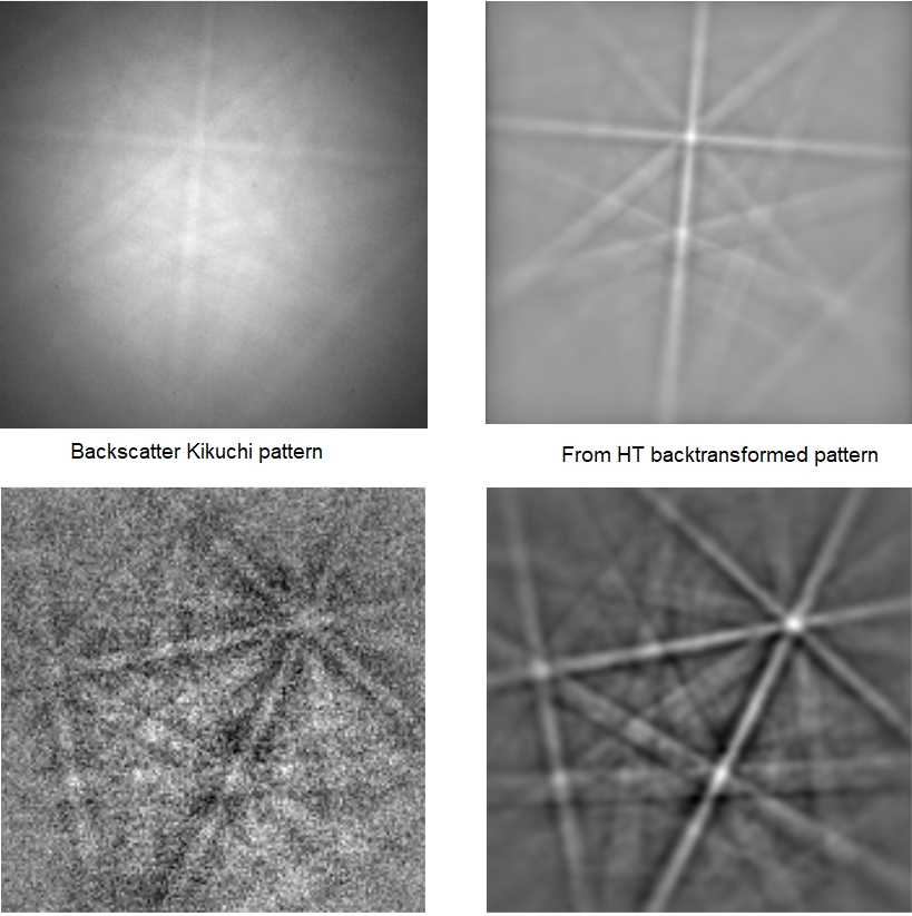
A near-pattern image can be reconstructed from the Radon transform using the back-projection operator, in a similar way to image reproduction as is common in computer tomography. The inverse transform specifies which straight line in the image space is associated with each cell in the Radon domain, and the stored intensity is equally attributed to all points on that line. The Radon backprojection does not provide the original image, but produces a smoothed image. In general, statistical noise is reduced. The Kikuchi bands in an originalpattern are bordered by slightly hyperbolic instead of straight lines.This may cause a further blur in back projection.
Applying a Radon transformation to the Kikuchi pattern simplifies the inherently difficult task of locating lines and bands, since only isolated peaks in the Radon domain need to be found. The "butterfly-like" peaks are best located by a peak search with constraints or by evaluating some coefficients of a 1D FFT of the Radon domain along ρ-direction. These peaks are assigned to Kikuchi bands in the pattern according to the inverse Radon transform [3]. 2b. The Hough Transformation Forty-five years after the publication of the Radon transformation, the Hough transformation was proposed by Paul V.C. Hough in a patent [4]. The underlying objective was to locate straight lines in a discrete image with binary intensity distribution fb(x, y), which originally represented particle tracks in a bubble chamber. The Hough transform is widely used in image processing to find edges and straight
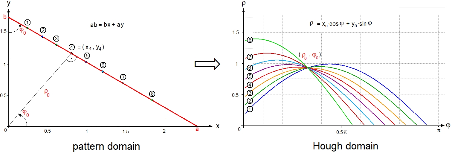
lines in binary images. It is more convenient to substitute the slope intercept parameterization of y = b - (b/a)× x , as specified in the original patent, with the polar parameterization of the straight line. The transformation from the image to the Hough domain then writes: If points (x, y) in the image lie on a straight line, their sinoidals intersect at a common point and their intensity is accumulated to a peak in the Hough domain.
In a binary image, pixels only take a value of either 1 or 0, so the value on each sinoidal is either 1 or 0. The Hough transform is a particularly fast method to locate sparse straight lines with isolated intensity values = 1, because pixels with intensity values = 0 are skipped during the transformation. Only for pixels with fb(x, y) = 1 the sinoidals are calculated and get intensity = 1. Thus, the height of the Hough peaks is equal to the number of intersecting sinoidals, i.e. the number of non-zero points on the corresponding line in the image. The discretization, inverse transform, and subsequent detection of bands are the same as described above for the Radon transform. Originally, the discrete Hough transform was defined only for binary (bitonal, 1-pixel) images. In a first step, grayscale images are converted to binary images by an edge filter before the Hough transform is carried out. Since Kikuchi patterns are gray-scale and not binary images, a Hough transform is, strictly speaking, not well suited for band detection. Of course, a gray-scale Kikuchi pattern can be reduced to a binary pattern, and then Hough transformed. The result is a significant loss of information, especially with respect to the band profile used to evaluate a meaningful Pattern Quality (PQ). On the other hand, the speed is increased by about a factor of 1/3, depending on the threshold of binarization (0 or 1) of the intensity levels. Another disadvantage of applying a Hough transform to binary Kikuchi patterns is a lower accuracy of orientation data. A better approach to increase speed, at the expense of accuracy, is to work with a higher binning rate, e.g. 60x60 pixels instead of 100x100 or more pixels per pattern. The discrete Hough transform was therefore "modified" in [5] to account for and evaluate gray-scale patterns. Thus the Hough transformation loses the advantage of high speed by skipping pixels with zero intensity. The result is quite similar to that of the direct Radon transformation without the run-length filter as discussed above. The theory and implementations of Radon and Hough transformations are presented in detail in [6, 7]. The Hough transformation and, moreover, its modification for grayscales are special cases of the Radon transformation. The essential difference between the Radon transform and the "modified" Hough transform in BKP analysis lies in the method of how the transformed domains are constructed from the image domain and rounding of values is carried out. In early EBSD analyses, peaks were located in the "Hough" domain by applying a normalized cross-correlation process with a large "butterfly-shaped" filter mask. In the simplest model, a rectangular pot profile was applied to the band intensity [5]. The main drawbacks of this method are the dependence of the band profile on the position of the band in the Kikuchi pattern, the type of pattern, the diffraction geometry, the accelerating voltage, the lattice type, and the {h k l} of the band to be detected. To satisfy this, the filter mask must be matched to the current band profile. Incorrectly matched masks will result in inaccurately determined band positions and bandwidths. The wider a band is, the larger the mask would have to be. Large masks increase the computing time extremely. A single mask is generally not sufficient; several masks are required to analyze a pattern. Overall, cross-correlation with a filter mask tends to be ineffective.
2c. Conclusion The inverse Radon transformation above is a way of looking at how a data point in Radon space is obtained from the pixels along a particular straight line (φ, ρ) in the image space of the Kikuchi pattern.The line is interrogated according to the intensities of the intersected pixels for accumulation. In contrast, the Hough transformation considers how each pixel in the image space of the Kikuchi pattern is mapped to the Hough space into a bundle of sinusoids representing all straight lines (φ, ρ) that intersect that pixel. They are all assigned the same pixel intensity. Finally, the sinusoids of all pixels are overlaid in Hough space and those related to dominant lines intersect in the form of butterfly shapes. The advantages of the Radon transformation include its conceptual simplicity and robustness. S is the path used for integration along the projection lines. For curves that are not straight lines, the natural extension is to project along the given curves, e.g., along hyperbolas, which are in fact the exact boundary lines of Kikuchi bands. The Hough formalism obscures the simplicity of the underlying transformation. The designation of Hough Transform, however, is prevalent in the EBSD literature, perhaps of not being aware of the history. The (inverse) Radon transform is ideal not only for parallel data processing on a GPU (Graphics Processor Unit) to unburden the CPU (Central Processor Unit) for band indexing and orientation calculations, but also for intelligent software with neural networks (AI). [2, 3] The general Radon transformation in Rn is an integral transformation that transforms a function f by integration along lines into a function Rf defined on the Rm. The Radon transformation has found a wide range of applications in digital image and signal processing [6]. Examples are electron microscopy of macromolecular assemblies such as viruses and protein complexes, barcode scanners, reflection seismology, and solving
hyperbolic partial differential equations. The ODF has been constructed from pole figures by Radon transformation [8], and the algorithm is implemented in the MTEX software package which is available for free [9]. The open-source software package PyEBSDIndex [10] is based on the Radon transform. An unprecedent speed of indexing several 10.000 patterns/sec is reported by performing the image processing calculations on the GPU rather than on the CPU. 3. A simple model of Radon peak profiles illustrates band detection as a constraint task
4. Peak verification by Artificial Neural Networks (ANN) Not all peaks in the Radon space that satisfy the constraints correspond to real bands in a diffraction pattern, since the underlying peak-shape model for band profile analysis is, in the interest of short execution time, as simple as possible and there are artifacts in Radon transforms. To increase the reliability of band extraction, a layered ANN was used to verify the detected bands [2]. ANN are superior to "sharp" verification methods based on numerical comparison of the shapes of actual and theoretical peaks, e.g., by checking a threshold value for the mean square deviation or by a cross-correlation test with a filter mask. The response function of a neuron is "soft" and "fuzzy". It can process a continuous range of intermediate values due to an adjustable sigmoid function. ANN can automatically "learn" complex relationships between data through training. They can be easily adjusted to many different peak profiles that are already present in one pattern, but in particular may vary significantly in general, especially with a change in material or phase, accelerating voltage, or diffraction set-up in general. A set of three-layer feed-forward neural networks with back-propagation (3L FFwBP) was implemented [2]:
[1] Download | |||||||||||||